Equated or linked tests need to share something. What do your tests share?
1. Items. Both tests have a few of the same items. (Common Item Equating)
2. Persons. Both tests were administered to a few of the same people. (Common Person Equating)
3. Person distribution. Both tests were administered to samples of people with the same ability distribution. (Common Distribution Equating)
4. Item content. Similar items in the two tests can be identified. (Common Item-Content "Virtual" Equating)
Test Equating and linking are usually straightforward with Winsteps, but do require clerical care. The more thought is put into test construction and data collection, the easier the equating will be.
Imagine that Test A (the more definitive test, if there is one) has been given to one sample of persons, and Test B to another. It is now desired to put all the items together into one item hierarchy, and to produce one set of measures encompassing all the persons.
Initially, analyze each test separately. Go down the "Diagnosis" pull-down menu. If the tests don't make sense separately, they won't make sense together.
There are several equating methods which work well with Winsteps. Test equating is discussed in Bond & Fox "Applying the Rasch model", and earlier in Wright & Stone, "Best Test Design".
"WINSTEPS-based Rasch methods that used multiple exam forms’ data worked better than Bayesian Markov Chain Monte Carlo methods, as the prior distribution used to estimate the item difficulty parameters biased predicted scores when there were difficulty differences between exam forms." Rasch Versus Classical Equating in the Context of Small Sample Sizes Ben Babcock and Kari J. Hodge. Educational and Psychological Measurement- Volume: 80, Number: 3 (June 2020)
We we want to put Test B onto Test A's scale. This is the same as putting Fahrenheit (Test B) temperatures onto a Celsius (Test A) scale:
New USCALE= for Test B = (Old USCALE= for Test B)*(S.D. of relevant persons or items for Test A)/(S.D. of relevant persons or items for Test B)
New UIMEAN= or UPMEAN= for Test B = (Mean of relevant persons or items for Test A) - ((Mean of relevant persons or items for Test B - Old UIMEAN or UPMEAN for Test B)*(S.D. of relevant persons or items for Test A)/(S.D. of relevant persons or items for Test B))
Rescaled Test B measure = ( (Old Test B measure - Old UIMEAN or UPMEAN for Test B)/(Old USCALE for Test B))*(New USCALE for Test B) + (New UIMEAN or UPMEAN for Test B)
Example: suppose we have freezing and boiling points in modified Fahrenheit and modified Celsius.
Test A: Celsius*200 + 50: USCALE=200, UIMEAN=50, freezing: 50, boiling: 20050, range = 20050-50 = 20000, mean = 10050
Test B: Fahrenheit*10+1000: USCALE=10, UIMEAN=1000, freezing: 1320, boiling: 3120, range = 3120-1320=1800, mean = 2220
For convenience, we will substitute the observed range for the S.D. in the equations above:
New Test B modified Fahrenheit USCALE = 10*20000/1800 = 111.1111
Then 1320, 3120 becomes (1320/10)*111.111 = 34666.7, (3120/10)*111.1111 = 14666.7,
so that the rescaled Test B range becomes 34666.7-14666.7 = 20000 = the Test A range
New Test B Fahrenheit UIMEAN = 10050 - (2220-1000)*20000/1800 = -3505.56
Thus, rescaled Test B freezing: 1320 becomes ((1320-1000)/10)*111.1111 - 3505.56 = 50 = Test A freezing
rescaled Test B boiling: 3120 becomes ((3120-1000)/10)*111.1111 - 3505.56 = 20050 = Test A boiling
Concurrent or One-step Equating
All the data are entered into one big array. This is convenient but has its hazards. Off-target items can introduce noise and skew the equating process, CUTLO= and CUTHI= may remedy targeting deficiencies. Linking designs forming long chains require much tighter than usual convergence criteria. Always cross-check results with those obtained by one of the other equating methods.
Concurrent equating of two tests, A and B, is usually easier than equating separate analyses. MFORMS= can help set up the data. But always analyze test A and test B separately first. Verify that test A and test B are functioning correctly. Then scatterplot the item difficulties for the common items from the separate analysis of Test A against the item difficulties from a separate analysis of Test B. Verify that they are on an approximately straight line approximately parallel to the identity line. Then do the concurrent analysis. You can also do a DIF analysis on the common items.
Example: 6 10-item Tests with some common persons between pairs of tests to form a chain linking all Tests. Groups of persons have also responded to each Test.
a) Use the content of the items, not the item statistics, to pair up a few items in each Test with their equivalents in one or more other Tests. Code this pairing into the item labels. These labels will act as indicators that the equating is working properly when we later list all 60 items in difficulty order. This is known as "virtual equating" - www.rasch.org/rmt/rmt193a.htm - We are not doing this to equate, but to validate the common-person equating, especially of Test 3.
b) Combine all the data into one Winsteps data file: 1,000 or so persons by 60 items. Put the Test number in the item labels, and the Group number in the person labels. Each student will have data for they tests they took and missing data for the tests they didn't take. The Winsteps MFORMS= instruction may help with this.
c) Run one analysis of everyone - "Concurrent equating".
Everything is in the same frame-of-reference
Every student has an ability measure, every Group has subtotals: Winsteps Table 28
Every item has a difficulty measure. Scan the list of 60 items in Measure order to check on (a). Any paired items that have conspicuously different difficulty measures deserve investigation. Every Test has subtotals, Winsteps Table 27.
DPF analysis of the common persons persons by Test indicates how stable person measures are across Tests: Winsteps Table 31.
This approach avoids having to make awkward (and error-prone) equating adjustments.
Common Item Equating
This is the best and easiest equating method. The two tests share items in common, preferably at least 5 spread out across the difficulty continuum. There is no specific minimum number of comon items. We usually want as many common items as possible, but are constrained by test design considerations. For instance, https://www.rasch.org/rmt/rmt51h.htm recommends 20 common items in each test. Great for tests of 200+ items, but what if the test only has 20 items in total? How low can we go? Only one common item is obviously too fragile. We can probably get away with 3 common items, spread across the ability range, but what if one or two of those items malfunction? So that leads us to 5 common items as a practical minimum. In a 20-item test (common in classroom tests), 5 items is one-quarter of the test. We would probably not want to go higher than one-quarter in order to limit item exposure and increase test security.
In the Winsteps analysis, indicate the common items with a special code in column 1 of the item labels.
Example: there are 6 items. Items 1 and 2 are common to the two tests. Items 3 and 4 are only in Test A. Items 5 and 6 are only in Test B
....
&END
C Item 1
C Item 2
A Item 3
A Item 4
B Item 5
B Item 6
END LABELS
Step 1. From the separate analyses,
obtain the mean and standard deviation of the common items:
use the "Specification" pull-down menu: ISUBTOT=1
Then produce Table 27 item summary statistics - this will give the mean and standard deviation of the common items.
Crossplot the difficulties of the common items, with Test B on the y-axis and Test A on the x-axis. The slope of the best fit is: slope = (S.D. of Test B common items) / (S.D. of Test A common items) i.e., the line through the point at the means of the common items and through the (mean + 1 S.D.). This should have a slope value near 1.0. If it does, then the first approximation: for Test B measures in the Test A frame of reference:
Measure (B) - Mean(B common items) + Mean(A common items) => Measure (A)
Step 2. Examine the scatterplot. Points far away from the best fit line indicate items that have behaved differently on the two occasions. You may wish to consider these to be no longer common items. Drop the items from the plot and redraw the best fit line. Items may be off the diagonal, or exhibiting large misfit because they are off-target to the current sample. This is a hazard of vertical equating. CUTLO= and CUTHI= may remedy targeting deficiencies.
Step 3a. If the best-fit slope remains far from 1.0, then there is something systematically different about Test A and Test B. You must do "Celsius - Fahrenheit" equating. Test A remains as it stands.
Include in the Test B control file:
USCALE = S.D. (A common items) / S.D.(B common items)
UMEAN = Mean(A common items) - Mean(B common items)
and reanalyze Test B. Test B is now in the Test A frame of reference, and the person measures from Test A and Test B can be reported together.
Note: This is computation is based on an approximate trend line through points measured with error ("error-in-variables").
Step 3b. The best-fit slope is near to 1.0. Suppose that Test A is the "benchmark" test. Then we do not want responses to Test B to change the results of Test A.
From a Test A analysis produce IFILE= and SFILE= (if there are rating or partial credit scales).
Edit the IFILE= and SFILE= to match Test B item numbers and rating (or partial credit) scale.
Use them as an IAFILE= and SAFILE= in a Test B analysis.
Test B is now in the same frame of reference as Test A, so the person measures and item difficulties can be reported together
Step 3c. The best-fit slope is near to 1.0. Test A and Test B have equal priority, and you want to use both to define the common items.
Use the MFORMS= command to combine the data files for Test A and Test B into one analysis. The results of that analysis will have Test A and Test B items and persons reported together.
Items
------------
||||||||||||
|||||||||||| Test A Persons
||||||||||||
||||||||||||
||||||||||||
||||||||||||
------------
- - - ------------
| | | ||||||||||||
| | | |||||||||||| Test B Persons
| | | ||||||||||||
| | | ||||||||||||
| | | ||||||||||||
| | | ||||||||||||
- - - ------------
Partial Credit items
"Partial credit" values are much less stable than dichotomies. Rather than trying to equate across the whole partial credit structure, one usually needs to assert that, for each item, a particular "threshold" or "step" is the critical one for equating purposes. Then use the difficulties of those thresholds for equating. This relevant threshold for an item is usually the transition point between the two most frequently observed categories - the Rasch-Andrich threshold - and so the most stable point in the partial credit structure.
Stocking and Lord iterative procedure
The Stocking and Lord (1983) present an iterative common-item procedure in which items exhibiting DIF across tests are dropped from the link until no items exhibiting inter-test DIF remain. A known hazard is that if the DIF distribution is skewed, the procedure trims the longer tail and the equating will be biased. To implement the Stocking and Lord procedure in Winsteps, code each person (in the person id label) according to which test form was taken. Then request a DIF analysis of item x person-test-code (Table 30). Drop items exhibiting DIF from the link, by coding them as different items in different tests.
Stocking and Lord (1983) Developing a common metric in item response theory. Applied Psychological Measurement 7:201-210.
Fuzzy Common-Item Equating
Two instruments measure the same trait, but with no items or persons in common.
1. Identify roughly similar pairs of items on the two instruments, and cross-plot their measures. We expect the plot to be fuzzy but it should indicate an equating line.
2. Virtual equating or pseudo-common-item equating (see below): Print the two item hierarchy maps and slide them up-and-down relative to each other until the overall item hierarchy makes the most sense. The relative placement of the local origins (zero points) of the two maps is the equating constant.
Choosing Common Items
1. Cross-plot the item difficulties of the pairs of possible common items from your original analyses.
2. In the scatterplot, there should be a diagonal line of items parallel to the identity line. These will be the best common items.
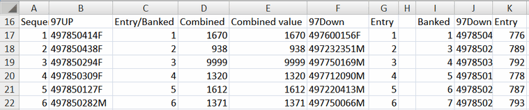
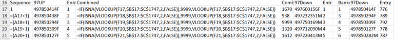
Common-item equating. Using Excel to construct a bank of item numbers for use with MFORMS=. Two test forms, 97Up and 97Down have some items in common. The item labels are in two Winsteps data files.
1. Copy the item labels from the Winsteps data files into this worksheet: Columns B and F
2. Put in sequence numbers in column A using =(cell above+1)
3. Copy Column A and paste special (values) into Columns C and G
4. In Column D, VLOOKUP Column F in Columns B, C. If #N/A then make it 9999
=IF(ISNA(VLOOKUP(F17,$B$17:$C$1747,2,FALSE)),9999,VLOOKUP(F17,$B$17:$C$1747,2,FALSE))
5. Copy column D and paste special (values) into Column E
6. Copy columns E F G into I J K
7. Sort IJK on columns I and K
8. Copy K into L
9. Go down column I to first 9999 (the first item in 97Down not in 97Up)
10. Place the first number after the last number in column A into column I
11. Sequence up from that number to the end of the items
12. The MFORMS= item-bank numbers for the first test are in column 1. They are the same as the original entry numbers.
13. The MFORMS= entry numbers for the second test are in column K. The bank numbers are in column I
Common Person Equating
Some persons have taken both tests, preferably at least 5 spread out across the ability continuum.
Step 1. From the separate analyses, crossplot the abilities of the common persons, with Test B on the y-axis and Test A on the x-axis. The slope of the best-fit line i.e., the line through the point at the means of the common persons and through the (mean + 1 S.D.) point should have slope near 1.0. If it does, then the intercept of the line with the x-axis is the equating constant.
First approximation: Test B measures in the Test A frame of reference = Test B measure + x-axis intercept.
Step 2. Examine the scatterplot. Points far away from the joint-best-fit trend-line indicate persons that have behaved differently on the two occasions. You may wish to consider these to be no longer common persons. Drop the persons from the plot and redraw the joint-best-fit trend-line.
Step 3a. If the best-fit slope remains far from 1.0, then there is something systematically different about Test A and Test B. You must do "Celsius - Fahrenheit" equating. Test A remains as it stands.
The slope of the best fit is: slope = (S.D. of Test B common persons) / (S.D. of Test A common persons)
Include in the Test B control file:
USCALE = the value of 1/slope
UMEAN = the value of the x-intercept
and reanalyze Test B. Test B is now in the Test A frame of reference, and the person measures from Test A and Test B can be reported together.
Step 3b. The best-fit slope is near to 1.0. Suppose that Test A is the "benchmark" test. Then we do not want responses to Test B to change the results of Test A.
From a Test A analysis produce PFILE=
Edit the PFILE= to match Test B person numbers
Use it as a PAFILE= in a Test B analysis.
Test B is now in the same frame of reference as Test A, so the person measures and person difficulties can be reported together
Step 3c. The best-fit slope is near to 1.0. Test A and Test B have equal priority, and you want to use both to define the common persons.
Use your text editor or word processor to append the common persons' Test B responses after their Test A ones, as in the design below. Then put the rest of the Test B responses after the Test A responses, but aligned in columns with the common persons's Test B responses. Perform an analysis of the combined data set. The results of that analysis will have Test A and Test B persons and persons reported together.
Test A items Test B items
|-----------------------------|
|-----------------------------|
|-----------------------------|
|-----------------------------||-----------------------------| Common Person
|-----------------------------|
|-----------------------------||-----------------------------| Common Person
|-----------------------------|
|-----------------------------|
|-----------------------------||-----------------------------| Common Person
|-----------------------------|
|-----------------------------|
|-----------------------------||-----------------------------| Common Person
|-----------------------------|
|-----------------------------|
|-----------------------------|
|-----------------------------|
|-----------------------------|
|-----------------------------|
|-----------------------------|
|-----------------------------|
|-----------------------------|
|-----------------------------|
|-----------------------------|
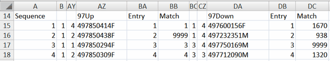
Common-person equating. Using Excel to construct a data file for use with Excel input. Two test forms, 97Up and 97Down have some person in common. The person labels are data are in Excel worksheets.
In a new worksheet
1. Copy test 1 responses and person labels to, say, columns B to AZ. The person labels are in AZ
2. Copy test 2 responses and person labels to, say, columns BC to DA. The person labels are in DA
3. Put in sequence numbers in column A using =(cell above+1)
4. Copy "values" column A to columns BA, DB
5. In column BB, VLOOKUP column AZ in column DA. If found BA, If not, 9999
=IF(ISNA(VLOOKUP(AZ15,$DA$15:$DB$1736,2,FALSE)),9999,BA15)
6. In column DC, VLOOKUP column DA in column AZ. If found the look-up value, If not, 9999
=IF(ISNA(VLOOKUP(DA15,$AZ$15:$BA$1736,2,FALSE)),9999,VLOOKUP(DA15,$AZ$15:$BA$1736,2,FALSE))
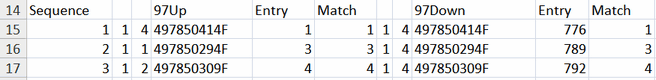
7. Sort B-BB on column BB, BA
8. Sort BC-DC on column DC, DB
9. Copy and paste the 9999 rows for Test 2 below the last row for Test 1
10. Use Winsteps Excel input to create a Winsteps control and data file for the combined data
Steps 1-6.
Steps 7-10.
Common Person Equating (or Subtests) with different Polytomies: An Example
400 persons have responded to Scale A (10 items) and Scale B (20 items). Scale A and Scale B have different rating scales.
I want a score-to-measure table for each Scale on the same measurement scale.
(1) Construct a data file with 400 rows (persons) and 30 columns (items)
10 items of scale A and 20 items of scale B
(2) define 2 rating scales, for the10 items of Scale A and the 20 items of Scale B.
ISGROUPS=*
1-10 A
11-30 B
*
(3) analyze all the data together with Winsteps
(4) Winsteps specification menu:
IDELETE=+1-10 ; notice the "+"
keeps Scale A items
(5) Output Table 20 for Scale A
(6) Winsteps specification menu:
IDELETE=
reinstates all items
IDELETE=1-10
deletes items for Scale A
(7) Output Table 20 for Scale B
Virtual Equating of Test Forms
The two tests share no items or persons in common, but the items cover similar material.
Step 1. Identify pairs of items of similar content and difficulty in the two tests. Be generous about interpreting "similar" at this stage. These are the pseudo-common items.
Steps 2-4: simple: The two item hierarchies (Table 1 using short clear item labels) are printed and compared, equivalent items are identified. The sheets of paper are moved vertically relative to each other until the overall hierarchy makes the most sense. The value on Test A corresponding to the zero on Test B is the UMEAN= value to use for Test B. If the item spacing on one test appear expanded or compressed relative to the other test, use USCALE= to compensate.
Or:
Step 2. From the separate analyses, crossplot the difficulties of the pairs of items, with Test B on the y-axis and Test A on the x-axis. The slope of the best-fit line i.e., the line through the point at the means of the common items and through the (mean + 1 S.D.) point should have slope near 1.0. If it does, then the intercept of the line with the x-axis is the equating constant.
First approximation: Test B measures in the Test A frame of reference = Test B measure + x-axis intercept.
Step 3. Examine the scatterplot. Points far away from the joint-best-fit trend-line indicate items that are not good pairs. You may wish to consider these to be no longer paired. Drop the items from the plot and redraw the trend line.
Step 4. The slope of the best fit is: slope = (S.D. of Test B common items) / (S.D. of Test A common items)
= Standard deviation of the item difficulties of the common items on Test B divided by Standard deviation of the item difficulties of the common items on Test A
Include in the Test B control file:
USCALE = the value of 1/slope
UMEAN = the value of the x-intercept
and reanalyze Test B. Test B is now in the Test A frame of reference, and the person and item measures from Test A and Test B can be reported together.
Random Equivalence Equating
The samples of persons who took both tests are believed to be randomly equivalent. Or, less commonly, the samples of items in the tests are believed to be randomly equivalent.
Step 1. From the separate analyses of Test A and Test B, obtain the means and sample standard deviation of the Rasch person-ability measures for two person samples (including extreme scores).
Step 2. To bring Test B into the frame of reference of Test A, adjust by the difference between the means of the Rasch person-ability measures for the person samples and user-rescale by the ratio of their sample standard deviations.
Include in the Test B control file:
USCALE = value of (sample S.D. person sample for Test A) / (sample S.D. person sample for Test B)
UMEAN = value of (mean for Test A) - (mean for Test B * USCALE)
and reanalyze Test B.
Check: Test B should now report the same sample mean and sample standard deviation as Test A for the Rasch person-ability measures.
Test B is now in the Test A frame of reference, and the person measures from Test A and Test B can be reported together.
In short::
1. Rasch-analyze each group separately.
2. Choose one group as the reference group. This is usually the largest group. Note down its group mean and S.D.
3. Adjust all the means and S.D. of the other groups so that they have the reference mean and S.D. - you can do this with UIMEAN= and USCALE=
4. Combine all the person files PFILE= and item files IFILE=. Excel files are convenient for this. Excel can sort etc.
Paired Item Equating - Parallel Items - Pseudo-Common Items
When constructing tests with overlapping content.
Step 1. From your list of items (or your two tests), choose 20 pairs of items. In your opinion, the difficulties of the two items in each pair should be approximately the same.
Step 2. One item of each pair is in the first test, and the other item is in the second test. Be sure to put codes in the item labels to remind yourself which items are paired.
Step 3. Collect your data.
Step 4. Analyze each test administration separately.
Step 5. Subtotal the difficulties of the paired items for each test administration (Table 27). The difference between the pair subtotals is the equating constant. Is this a reasonable value? You can use this value in UIMEAN= of one test to align the two tests.
Step 6.Cross-plot the difficulties of the pairs of items (with confidence bands computed from the standard errors of the pairs of item estimates). The plot will confirm (hopefully) your opinion about the pairs of item difficulties. If not, you will learn a lot about your items!!
Linking Tests with Common Items
Here is an example:
A. The first test (50 items, 1,000 students)
B. The second test (60 items, 1,000 students)
C. A linking test (20 items from the first test, 25 from the second test, 250 students)
Here is a typical Rasch approach. It is equivalent to applying the "common item" linking method twice.
(a) Rasch analyze each test separately to verify that all is correct.
(b) Cross-plot the item difficulties for the 20 common items between the first test and the linking test. Verify that the link items are on a statistical trend line parallel to the identity line. Omit from the list of linking items, any items that have clearly changed relative difficulty. If the slope of the trend line is not parallel to the identity line (45 degrees), then the test discrimination has changed. The test linking will use a "best fit to trend line" conversion:
Corrected measure on test 2 in test 1 frame-of-reference =
((observed measure on test 2 - mean measure of test 2 link items)*(SD of test 1 link items)/(SD of test 1 link items))
+ mean measure of test 1 link items
(c) Cross-plot the item difficulties for the 25 common items between the second test and the linking test. Repeat (b).
(d1) If both trend lines are approximately parallel to the identity line, than all three tests are equally discriminating, and the simplest equating is "concurrent". Put all 3 tests in one analysis. You can use the MFORMS= command to put all items into one analysis. You can also selectively delete items using the Specification pull-down menu in order to construct measure-to-raw score conversion tables for each test, if necessary.
Or you can use a direct arithmetical adjustment to the measures based on the mean differences of the common items: www.rasch.org/memo42.htm "Linking tests".
(d2) If best-fit trend lines are not parallel to the identity line, then tests have different discriminations. Equate the first test to the linking test, and then the linking test to the second test, using the "best fit to trend line" conversion, shown in (b) above. You can also apply the "best fit to trend" conversion to Table 20 to convert every possible raw score.
