the rating scale for each item is analyzed as a set of consecutive dichotomies with one dichotomy for each category boundary, CDM - Consecutive Dichotomies Model. This is similar to MSD, see Bradley C., Massof R. (2018) Method of successive dichotomizations: An improved method for estimating measures of latent variables from rating scale data. PLoS One.
Similarly to MSD, "consecutive dichotomies" replaces the rating scale with a set of dichotomous items. This was one of the ways that rating scales were analyzed before David Andrich devised his model in 1977. Dichotomization of rating scales has recently been reintroduced because of its conveniences. An effect of this dichotomization is to widen the logit range of the measures. In the example analysis below , the Andrich range is 1.4 logits, but the dichotomized range is 3.2 logits. So, if you are using a rule such as "DIF begins at 0.5 logits" then more instances of DIF will be reported with dichotomization than with the Andrich model. Accordingly, we need to adjust the DIF criteria to match the new situation.
Suggestion: identify DIF in a dataset with the Andrich model. Reanalyze with consecutive dichotomies. You will now be able to construct DIF criteria for the MSD situation which match the Andrich situation. If you do this, please do write a short research note about this for publication in Rasch Measurement Transactions or inclusion in Winsteps Help and, of course, there are many Journals where you could publish a larger paper about this.
MSD vs. Consecutive Dichotomies Model, CDM:
MSD: Chris Bradley emailed me on 4-4-2025: "Regarding the approximation technique (the implemented MSD code in R), the concept is quite simple. Let’s say the rating scale has 5 categories, so 4 thresholds. MSD dichotomizes the rating scale data for each threshold and applies the original dichotomous Rasch model to each dichotomization. The result in this case is 4 sets of estimated person and item measures. If there [is no missing data] in any set of item or person measures, the average of the 4 sets gives you the final set of MSD person and item measures. Once person and item measures are estimated, each threshold is estimated one at a time using the corresponding dichotomized data (only one unknown remains once all person and item measures are fixed)."
CDM: estimation is done with a tweak of Masters' PCM algorithm. PCM compares frequencies of adjacent categories for an item. Consecutive dichotomies compare frequencies of all categories above with all categories below each threshold for an item. Thus each original item is equivalent to a set of dichotomous items estimated together in one analysis.
Andrich RSM, Masters' PCM and polytomous PROX are difficult to explain to the non-technical. In the Masters' PCM, the threshold (category) parameters for each item are determined by the relative frequencies of the category immediately above vs. the frequency of the category immediately below each threshold of the rating scale. In the Consecutive Dichotomization Model, CDM, the parameters are determined by the frequencies of all categories above vs. all categories below the threshold for the rating scel of each item. CDM makes the parameters immediately interpretable on the latent variable as category boundaries (unlike RSM or PCM). There are no disordered thresholds. Categories can be split or combined without altering the relationships between the other thresholds. In RSM or PCM, splitting or combining categories changes the relationships between all the thresholds.
The Andrich Rating-Scale Model, the Masters' Partial Credit Model and the Linacre Grouped-Rating-Scale Model can all be written in this way:
|
(1) |
where Fk indicates RSM, which can be written as Fik for PCM and Fgk for GRSM with Dgi where g indicates the item belongs to item-group g. The number of categories is m+1, and F0 = 0 or any convenient constant (it cancels out of the algebra).
Equation (1) hides the fundamental structure of these Rasch models, which is revealed when we rewrite this equation in logit-linear form:
|
(2) |
We can see here the simple additive (linear) form of a Rasch model so that each parameter has a "sufficient statistic" (= raw score or count in the data).
We can write the CDM model in the same way conceptually. This is not an exact algebraic representation of the CDM model. The Pnij values are inferred from the frequency of the categories, 0 to m, in the data.
|
(3) |
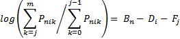
with the same options for Fj as RSM, PCM and GRSM. Then the CDM thresholds correspond to a sequence of dichotomized items of equal or ascending difficulty, Fj >= Fj-1.
In practical terms,CDM is similar to the Samejima (1969) Graded Response Model with discrimination set to 1.0.
Pni0 is the probability of failing the easiest dichotomy.
|
(10) |
Pni1 is the probability of failing the second easiest dichotomy, but not failing the easiest dichotomy. This probability must be greater or equal to zero because the dichotomies are ordered.
|
(11) |
Pni2 is the probability of failing the third easiest dichotomy, but not failing the easier dichotomies,
|
(12) |
and so until the incremental probability of failing all the dichotomies is known. Then the probability of succeeding on the most difficult dichotomy, m, is the remaining probability Pnim.
|
(13) |
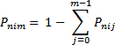
The reported person and item Standard Errors for CDM are estimated the same way as PCM.
See Example at Models-