Please explain Rasch PCA of Residuals in plain English for people like me who are not particularly good at mathematical terminology.
Rasch "PCA of residuals" looks for patterns in the part of the data that does not accord with the Rasch measures. This is the "unexpected" part of the data. We are looking to see if groups of items share the same patterns of unexpectedness. If they do, then those items probably also share a substantive attribute in common, which we call a "secondary dimension". Then our questions are:
1. "What is the secondary dimension?" - to discover this we look at the contrast between the content of the items at the top, A,B,C, and the bottom, a,b,c, of the contrast plot in Table 23.2. For instance, if the items at the top are "physical" items and the items at the bottom are "mental" items. Then there is a secondary dimension with "physical" at one end, and "mental" at the other.
2. "Is the secondary dimension big enough to distort measurement?" - usually the secondary dimension needs to have the strength of at least two items to be above the noise level. We see the strength (eigenvalue) in the first column of numbers in Table 23.0.
3. "What do we do about it?" - often our decision is "nothing". On a math test, we will get a big contrast between "algebra" and "word problems". We know that they are conceptually different, but they are both part of math. We don't want to omit either of them, and we don't want separate "algebra" measures and "word problem" measures. So the best we can do is to verify that the balance between the number of algebra items and the number of word-problem items is in accordance with our test plan.
But we may see that one end of the contrast is off-dimension. For instance, we may see a contrast between "algebra items using Latin letters" and "algebra items using Greek letters". We may decide that knowledge of Greek letters is incidental to our purpose of measuring the understanding of algebraic operations, and so we may decide to omit or revise the Greek-letter items.
In summary: Look at the content (wording) of the items at the top and bottom of the contrast: items A,B,C and items a,b,c. If those items are different enough to be considered different dimensions (similar to "height" and "weight"), then split the items into separate analyses. If the items are part of the same dimension (similar to "addition" and "subtraction" on an arithmetic test), then no action is necessary. You are seeing the expected co-variance of items in the same content area of a dimension.
For more discussion see Dimensionality: when is a test multidimensional?
For technical details:
For residuals, see www.rasch.org/rmt/rmt34e.htm
For PCA, builtin.com/data-science/step-step-explanation-principal-component-analysis and many other websites
For the "Variance explained by ...", see www.rasch.org/rmt/rmt173g.htm
Principal-Components Analysis of Residuals is not interpreted in the same way as Common-Factor Analysis of the original data.
In Common-Factor analysis, we try to optimize the commonalities, maximization, rotation and obliqueness to give the strongest possible factor structure, where the unstandardized "raw" factor loadings are interpreted as the correlations with the latent factors.
In PCA of residuals, we are trying to falsify the hypothesis that the residuals are random noise by finding the component that explains the largest possible amount of variance in the residuals. This is the "first contrast" (or first PCA component in the correlation matrix of the residuals). If the eigenvalue of the first contrast is small (usually less than 2.0) then the first contrast is at the noise level and the hypothesis of random noise is not falsified in a general way. If not, the loadings on the first contrast indicate that there are contrasting patterns in the residuals. The absolute sizes of the loadings are generally inconsequential. It is the patterns of the loadings that are important. We see the patterns by looking at the plot of the loadings in Winsteps Table 23.2, particularly comparing the top and bottom of the plot.
So, if we notice that the 1st contrast has an eigenvalue of 3 (the strength of 3 items), and we see on the contrast plot that there is a group of 3 items (more or less) outlying toward the top or the bottom of the plot, then we attribute the first contrast to the fact that their pattern contrasts with the pattern of the other items. We then look at the content of those items to discover what those items share that contrasts with the content of the other items.
Please do not interpret Rasch-residual-based Principal Components Analysis (PCAR) as a usual factor analysis. These components show contrasts between opposing factors, not loadings on one factor. Criteria have yet to be established for when a deviation becomes a dimension. So PCA is indicative, but not definitive, about secondary dimensions.
In conventional factor analysis, interpretation may be based only on positive loadings. In the PCA of Residuals, interpretation must be based on the contrast between positive and negative loadings.
The "first factor" (in the traditional Factor Analysis sense) is the Rasch dimension. By default all items (or persons) are in the "first factor" until proven otherwise. The first contrast plot shows a contrast within the data between two sets of items orthogonal to the Rasch dimension. We usually look at the plot and identify a cluster of items at the top or bottom of the plot which share most strongly some substantive off-Rasch-dimension attribute. These become the "second factor".
Winsteps is doing a PCA of residuals, not of the original observations. So, the first component (dimension) has already been removed. We are looking at secondary dimensions, components or contrasts. When interpreting the meaning of a component or a factor, the conventional approach is only to look at the largest positive loadings in order to infer the substantive meaning of the component. In Winsteps PCA this method of interpretation can be misleading, because the component is reflecting opposing response patterns across items by persons. So we need to identify the opposing response patterns and interpret the meaning of the component from those. These are the response patterns to the items at the top and bottom of the plots.
Sample size: A useful criterion is 100 persons for PCA of items, and 100 items for PCA of persons, though useful findings can be obtained with 20 persons for PCA of items, and 20 items for PCA of persons.
Arrindell, W. A., & van der Ende. J. (1985). An empirical test of the utility of the observations-to-variables ratio in factor and components analysis. Applied Psychological Measurement, 9, 165 - 178.
Compatibility with earlier computation: The Winsteps algorithm was changed to align more closely with the usual practice in statistics of explaining raw-score variance (parallel to Outfit). The earlier method in Winsteps was explaining the statistical-information variance (parallel to Infit). Since the outlying observations have high raw-score variance, but low statistical-information variance, the previous computation showed Rasch explaining a higher proportion of the variance.
If you want to do a more conventional interpretation, then output the ICORFIL= correlation matrix from the Output Files menu. You can read this into a factor analysis program, such as SAS or SPSS. You can then do a PCA or CFA (common factor analysis) of the correlation matrix, with the usual obliquenesses, rotations etc.
In Winsteps, you can also do a PCA of the original observations by specifying PRCOMP=Obs
Example from Table 23.0 from Example0.txt:
Table of STANDARDIZED RESIDUAL variance (in Eigenvalue units)
-- Observed -- Expected
Total raw variance in observations = 51.0 100.0% 100.0%
Raw variance explained by measures = 26.0 51.0% 50.8%
Raw variance explained by persons = 10.8 21.2% 21.2%
Raw Variance explained by items = 15.1 29.7% 29.6%
Raw unexplained variance (total) = 25.0 49.0% 100.0% 49.2%
Unexplned variance in 1st contrast = 4.6 9.1% 18.5%
Unexplned variance in 2nd contrast = 2.9 5.8% 11.8%
Unexplned variance in 3rd contrast = 2.3 4.5% 9.2%
Unexplned variance in 4th contrast = 1.7 3.4% 6.9%
Unexplned variance in 5th contrast = 1.6 3.2% 6.5%
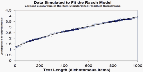
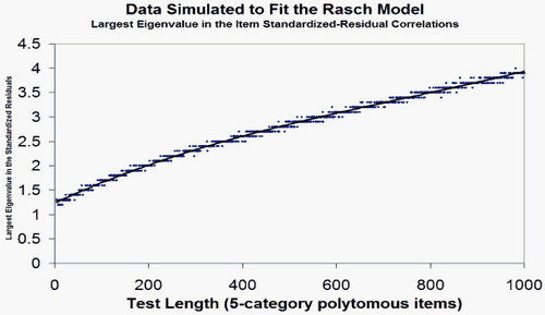
The Rasch dimension explains 51.0% of the variance in the data: good! The largest secondary dimension, "the first contrast in the residuals" explains 9.1% of the variance - somewhat greater than around 4% that would be observed in data like these simulated to fit the Rasch model. Check this by using the SIMUL= option in Winsteps to simulate a Rasch-fitting dataset with same characteristics as this dataset. Then produce this Table 23 for it. Also see: www.rasch.org/rmt/rmt191h.htm
In these data, the variance explained by the items, 29.7% is only three times the variance explained by the first contrast 9.1%, so there is a noticeable secondary dimension in the items. The eigenvalue of the first contrast is 4.6 - this indicates that it has the strength of about 5 items (4.6 rounded to 5, out of 25), somewhat bigger than the strength of two items (an eigenvalue of 2), the smallest amount that could be considered a "dimension". Contrast the content of the items at the top and bottom of the plot in Table 23.2 to identify what this secondary dimension reflects.
Tentative guidelines:
1. Is your person measure S.D. in Table 3 what you expect (or better)?
Yes, then your "variance explained by persons"is also good.
2. 1. Is your item difficulty S.D. in Table 3 what you expect (or better)?
Yes, then your "variance explained by the items" is also good.
3. Is your unexplained variance explained by 1st contrast (eigenvalue size) < 2.0 ?
Yes, then your biggest secondary dimension has the strength of less than 2 items. Good. For the expected size of the unexplained variance:
4. Now, please simulate Rasch-fitting data like yours, and compare Table 23 and Table 24 with it.
There is a paradox: "more variance explained" ® "more unidimensional" in the Guttman sense - where all unexplained variance is viewed as degrading the perfect Guttman uni-dimension. But "more unidimensional" (in the stochastic Rasch sense) depends on the size of the second dimension in the data, not on the variance explained by the first (Rasch) dimension. This is because most unexplained variance is hypothesized to be the random noise predicted by the Rasch model, rather than a degradation of the unidimensionality of the Rasch measures
Analytical Note:
Winsteps performs an unrotated "principal components" factor analysis. (using Hotelling's terminology). If you would like to rotate axes, have oblique axes, or perform a "common factor" factor analysis of the residuals, Winsteps can write out the matrices of residual item (or person) correlations, see the "Output Files" pull down menu or ICORFIL= and PCORFIL=. You can import these into any statistics software package.
The purpose of PCA of residuals is not to construct variables (as it is with "common factor" analysis), but to explain variance. First off, we are looking for the contrast in the residuals that explains the most variance. If this contrast is at the "noise" level, then we have no shared second dimension. If it does, then this contrast is the "second" dimension in the data. (The Rasch dimension is hypothesized to be the first). Similarly we look for a third dimension, etc. Rotation, oblique axes, the "common factor" approach, all reapportion variance, usually in an attempt to make the factor structure more clearly align with the items, but, in so doing, the actual variance structure and dimensionality of the data is masked.
In Rasch analysis, we are trying to do the opposite of what is usually happening in factor analysis. In Rasch analysis of residuals, we want not to find contrasts, and, if we do, we want to find the least number of contrasts above the noise level, each, in turn, explaining as much variance as possible. This is exactly what unrotated PCA does.
In conventional factor analysis of observations, we are hoping desperately to find shared factors, and to assign the items to them as clearly and meaningfully as possible. In this endeavor, we use a whole toolbox of rotations, obliquenesses and choices of diagonal self-correlations (i.e., the "common factor" approach).
But, different analysts have different aims, and so Winsteps provides the matrix of residual correlations to enable the analyst to perform whatever factor analysis is desired!
The Rasch Model: Expected values, Model Variances, and Standardized Residuals
The Rasch model constructs additive measures from ordinal observations. It uses disordering of the observations across persons and items to construct the additive frame of reference. Perfectly ordered observations would accord with the ideal model of Louis Guttman, but lack information as to the distances involved.
Since the Rasch model uses disordering in the data to construct distances, it predicts that this disordering will have a particular ideal form. Of course, empirical data never exactly accord with this ideal, so a major focus of Rasch fit analysis is to discover where and in what ways the disordering departs from the ideal. If the departures have substantive implications, then they may indicate that the quality of the measures is compromised.
A typical Rasch model is:
log (Pnik / Pni(k-1) ) = Bn - Di - Fk
where
Pnik = the probability that person n on item i is observed in category k, where k=0,m
Pni(k-1) = the probability that person n on item i is observed in category k-1
Bn = the ability measure of person n
Di = the difficulty measure of item i
Fk = the structure calibration from category k-1 to category k
This predicts the observation Xni. Then
Xni = Eni ± sqrt(Vni)
where
Eni = sum (kPnik) for k=0,m.
This is the expected value of the observation.
Vni = sum (k²Pnik) - (Eni)² for k=0,m.
This is the model variance of the observation about its expectation, i.e., the predicted randomness in the data.
The Rasch model is based on the specification of "local independence". This asserts that, after the contribution of the measures to the data has been removed, all that will be left is random, normally distributed. noise. This implies that when a residual, (Xni - Eni), is divided by its model standard deviation, it will have the characteristics of being sampled from a unit normal distribution. That is:
(Xni - Eni) / sqrt (Vni), the standardized residual of an observation, is specified to be N(0,1)
The bias in a measure estimate due to the misfit in an observation approximates (Xni - Eni) * S.E.²(measure)
Principal Components Analysis of Residuals
"Principal Component Analysis (PCA) is a powerful technique for extracting structure from possibly high-dimensional data sets. It is readily performed by solving an eigenvalue problem, or by using iterative algorithms which estimate principal components [as in Winsteps]. ... some of the classical papers are due to Pearson (1901); Hotelling (1933); ... PCA is an orthogonal transformation of the coordinate system in which we describe our data. The new coordinate values by which we represent the data are called principal components. It is often the case that a small number of principal components is sufficient to account for most of the structure in the data. These are sometimes called factors or latent variables of the data." (Schölkopf, D., Smola A.J., Müller K.-R., 1999, Kernel Principal Component Analysis, in Schölkopf at al. "Advances in Kernel Methods", London: MIT Press).
Pearson, K. (1901) On lines and planes of closest fit to points in space. Philosophical Magazine, 2:559-572.
Hotelling, H. (1933) Analysis of a complex of statistical variables into principal components. Journal of Educational Psychology, 24:417-441, 498-520.
The standardized residuals are modeled to have unit normal distributions which are independent and so uncorrelated. A PCA of Rasch standardized residuals should look like a PCA of random normal deviates. Simulation studies indicate that the largest component would have an eigenvalue of about 1.4 and they get smaller from there. But there is usually something else going on in the data, so, since we are looking at residuals, each component contrasts deviations in one direction ("positive loading") against deviation in the other direction ("negative loading"). As always with factor analysis, positive and negative loading directions are arbitrary. Each component in the residuals only has substantive meaning when its two ends are contrasted. This is a little different from PCA of raw observations where the component is thought of as capturing the "thing".
Loadings are plotted against Rasch measures because deviation in the data from the Rasch model is often not uniform along the variable (which is actually the "first" dimension). It can be localized in easy or hard items, high or low ability people. The Wright and Masters "Liking for Science" data is an excellent example of this.
Total, Explained and Unexplained Variances
The decomposition of the total variance in the data set proceeds as follows for the standardized residual, PRCOMP=S and raw score residual PRCOMP=R, option.
(i) The average person ability measure, b, and the average item difficulty measure, d, are computed.
(ii) The expected response, Ebd, by a person of average ability measure to an item of average difficulty measure is computed. (If there are multiple rating or partial credit scales, then this is done for each rating or partial credit scale.)
(iii) Each observed interaction of person n, of estimated measure Bn, with item i, of estimated measure Di, produces an observation Xni, with an expected value, Eni, and model variance, Vni.
The raw-score residual, Zni, of each Xni is Zni = Xni-Eni.
The standardized residual, Zni, of each Xni is Zni = (Xni-Eni)/sqrt(Vni).
Empirically:
(iv) The piece of the observation available for explanation by Bn and Di is approximately Xni - Ebd.
In raw-score residual units, this is Cni = Xni-Ebd
In standardized residual units, this is Cni = (Xni-Ebd)/sqrt(Vni)
The total variance sum-of-squares in the data set available for explanation by the measures is: VAvailable = sum(Cni²)
(v) The total variance sum of squares predicted to be unexplained by the measures is: VUnexplained = sum(Zni²)
(vi) The total variance sum of squares explained by the measures is: VExplained = VAvailable - VUnexplained
If VEXplained is negative, see below.
Under model conditions:
(viii) The total variance sum of squares explained by the measures is:
Raw-score residuals: VMexplained = sum((Eni-Ebd)²)
Standardized residuals: VMexplained = sum((Eni-Ebd)²/Vni)
(ix) The total variance sum of squares predicted to be unexplained by the measures is:
Raw score residuals: VMunexplained = sum(Vni)
Standardized residuals: VMunexplained = sum(Vni/Vni) = sum(1)
x) total variance sum-of-squares in the data set predicted to be available for explanation by the measures is: VMAvailable = VMexplained + VMUnexplained
Negative Variance Explained
Table of STANDARDIZED RESIDUAL variance (in Eigenvalue units)
Total variance in observations = 20.3 100.0%
Variance explained by measures = -23.7 -116.2%
According to this Table, the variance explained by the measures is less than the theoretical minimum of 0.00. This "negative variance" arises when there is unmodeled covariance in the data. In Rasch situations this happens when the randomness in the data, though normally distributed when considered overall, is skewed when partitioned by measure difference. A likely explanation is that some items are reverse-coded. Check that all correlations are positive by viewing the Diagnosis Menu, Table A. If necessary, use IREFER= to recode items. If there is no obvious explanation, please email your control and data file to www.winsteps.com
Principal Components Analysis of Standardized Residuals
(i) The standardized residuals for all observations are computed. Missing observations are imputed to have a standardized residual of 0, i.e., to fit the model.
(ii) Correlation matrices of standardized residuals across items and across persons are computed. The correlations furthest from 0 (uncorrelated) are reported in Tables 23.99 and 24.99.
(iii) In order to test the specification that the standardized residuals are uncorrelated, it is asserted that all randomness in the data is shared across the items and persons. This is done by placing 1's in the main diagonal of the correlation matrix. This accords with the "Principal Components" approach to Factor Analysis. ("General" Factor Analysis attempts to estimate what proportion of the variance is shared across items and persons, and reduces the diagonal values from 1's accordingly. This approach contradicts our purpose here.)
(iv) The correlation matrices are decomposed. In principal, if there are L items (or N persons), and they are locally independent, then there are L item components (or N person components) each of size (i.e., eigenvalue) 1, the value in the main diagonal. But there are expected to be random fluctuations in the structure of the randomness. However, eigenvalues of less than 2 indicate that the implied substructure (dimension) in these data has less than the strength of 2 items (or 2 persons), and so, however powerful it may be diagnostically, it has little strength in these data.
(v) If items (or persons) do have commonalities beyond those predicted by the Rasch model, then these may appear as shared fluctuations in their residuals. These will inflate the correlations between those items (or persons) and result in components with eigenvalues greater than 1. The largest of these components is shown in Table 23.2 and 24.3, and sequentially smaller ones in later subtables.
(vi) In the Principal Components Analysis, the total variance is expressed as the sum of cells along the main diagonal, which is the number of items, L, (or number of persons, N). This corresponds to the total unexplained variance in the dataset, VUnexplained.
(vii) The variance explained by the current contrast is its eigenvalue.
Sample size: The more, the better .,...
"There are diminishing returns, but even at large subject to item ratios and sample sizes (such as 201 ratio or N > 1000) and with unrealistically strong factor loadings and clear factor structures, EFA and PCA can produce error rates up to 30%, leaving room for improvement via larger samples." Osborne, Jason W. & Anna B. Costello (2004). Sample size and subject to item ratio in principal components analysis. scholarworks.umass.edu/pare/vol9/iss1/11/
Example: Item Decomposition
From Table 23.2: The Principal Components decomposition of the standardized residuals for the items, correlated across persons. Winsteps reports:
Table of STANDARDIZED RESIDUAL variance (in Eigenvalue units)
Empirical Modeled
Total variance in observations = 1452.0 100.0% 100.0%
Variance explained by measures = 1438.0 99.0% 98.6%
Unexplained variance (total) = 14.0 1.0% 1.4%
Unexpl var explained by 1st contrast = 2.7 .2%
The first contrast has an eigenvalue size of 2.7 This corresponds to 2.7 items.
There are 14 active items, so that the total unexplained variance in the correlation matrix is 14 units.
The "Modeled" column shows what this would have looked like if these data fit the model exactly.
Conclusion: Though this contrast has the strength of 3 items, and so might be independently constructed from these data, its strength is so small that it is barely a ripple on the total measurement structure.
Caution: The 1st contrast may be an extra dimension, or it may be a local change in the intensity of this dimension:
Table of STANDARDIZED RESIDUAL variance (in Eigenvalue units)
Empirical Modeled
Total variance in observations = 97.1 100.0% 100.0%
Variance explained by measures = 58.1 59.8% 59.0%
Unexplained variance (total) = 39.0 40.2% 100.0% 41.0%
Unexpl var explained by 1st contrast = 2.8 2.9% 7.2%
-3 -2 -1 0 1 2 3
++----------+----------+----------+----------+----------+----------++ COUNT
| | A | 1
.7 + | +
| | B C | 2
F .6 + | +
A | | D | 1
C .5 + E | + 1
T | | |
O .4 + | +
R | | |
.3 + | +
1 | F | | 1
.2 + | +
L | | G | 1
O .1 + H | + 1
A | L I | J K | 4
D .0 +----------M-----------------N----|-O-------------------------------+ 3
I | T S QR | P s | 6
N -.1 + p o| q r + 4
G | | l m n k | 4
-.2 + i g | jh + 4
| f c e |b d | 5
-.3 + | +
| a | | 1
++----------+----------+----------+----------+----------+----------++
-3 -2 -1 0 1 2 3
Item MEASURE
+-----------------------------------------
|CON- | RAW | INFIT OUTFIT| ENTRY
| TRAST|LOADING|MEASURE MNSQ MNSQ |NUMBER
|------+-------+-------------------+------
| 1 | .74 | .71 .78 .70 |A 26
| 1 | .65 | .26 .79 .68 |B 23
| 1 | .64 | 1.34 .87 .84 |C 25
| 1 | .56 | .64 .85 .80 |D 24
| 1 | .51 | -.85 .84 .60 |E 22
The first contrast comprises items A-E. But their mean-squares are all less than 1.0, indicating they do not contradict the Rasch variable, but are rather too predictable. They appear to represent a local intensification of the Rasch dimension, rather than a contradictory dimension.
Comparison with Rasch-fitting data
Winsteps makes it easy to compare empirical PCA results with the results for an equivalent Rasch-fitting data set.
From the Output Files menu, make a "Simulated Data" file, call it, say, test.txt
From the Files menu, Restart Winsteps. Under "Extra specifications", type in "data=test.txt".
Exactly the same analysis is performed, but with Rasch-fitting data. Look at the Dimensionality table:
Table of STANDARDIZED RESIDUAL variance (in Eigenvalue units)
Empirical Modeled
Total variance in observations = 576.8 100.0% 100.0%
Variance explained by measures = 562.8 97.6% 97.1%
Unexplained variance (total) = 14.0 2.4% 2.9%
Unexpl var explained by 1st contrast = 2.2 .4%
Repeat this process several times, simulating a new dataset each time. If they all look like this, we can conclude that the value of 2.7 for the 1st contrast in the residuals is negligibly bigger than the 2.2 expected by chance.
General Advice
A question here is "how big is big"? Much depends on what you are looking for. If you expect your instrument to have a wide spread of items and a wide spread of persons, then your measures should explain most of the variance. But if your items are of almost equal difficulty (as recommended, for instance, by G-Theory) and your persons are of similar ability (e.g., hospital nurses at the end of their training) then the measures will only explain a small amount of the variance.
Winsteps Table 23.6 implements Ben Wright's recommendation that the analyst split the test into two halves, assigning the items, top vs. bottom of the first component in the residuals. Measure the persons on both halves of the test. Cross-plot the person measures. If the plot would lead you to different conclusions about the persons depending on test half, then there is a multidimensionality. If the plot is just a fuzzy straight line, then there is one, perhaps somewhat vague, dimension.
Tentative guidelines:
Please look the nomogram above from https://www.rasch.org/rmt/rmt221j.htm - it indicates the expected relationship between "explained variance" and "unexplained variance". 40%-50% are typical values.
In the unexplained variance, a "secondary dimension" must have the strength of at least 3 items, so if the first contrast has "units" (i.e., eigenvalue) less than 3 (for a reasonable length test) then the test is probably unidimensional. (Of course, individual items can still misfit).
Negative variance can occur when the unexpectedness in the data is not random. An example is people who flat-line an attitude survey. Their unexpected responses are always biased towards one category of the rating (or partial credit) scale.
Simulation studies indicate that eigenvalues less than 1.4 are at the random level. Smith RM, Miao CY (1994) Assessing unidimensionality for Rasch measurement. Chapter 18 in M. Wilson (Ed.) Objective Measurement: Theory into Practice. Vol. 2. Norwood NJ: Ablex.) On occasion, values as high as 2.0 are at the random level. (Critical Eigenvalue Sizes in Standardized Residual Principal Components Analysis, Raîche G., Rasch Measurement Transactions, 2005, 19:1 p. 1012.)
To compute these numbers yourself ...
Let's assume we have a complete dichotomous dataset of N persons and L items. Then, in summary,
1. Do the Rasch analysis. Write out the raw observations, the raw residuals, and the standardized residuals
2. Compute the observed variance of the raw observations = OV = 100% of the variance in the data
3. Compute the unexplained variance = mean-square (raw residuals) = UV = Unexplained %
4. Compute the explained variance in the raw observations = OV-UV = EV = Explained % (can go negative!)
5. The eigenvalue of the item inter-correlation matrix of the standardized residuals = L = UV (rescaled) = Unexplained %
6. In the decomposition of the correlation matrix: Eigenvalue of the component (factor) = G = "strength in item units" = Unexplained% * Number of items
For the plots, the item difficulties are the x-axis, and the component loadings as the y-axis. This is a reminder that the Rasch dimension is the implicit first dimension in the original observations.
You will notice that some of this is statistically approximate, but more exact statistics have produced less meaningful findings. Together with Albert Einstein, trust the meaning more than the numbers!
Will Table 23 work with CMLE=Yes values?
Suppose I anchor IAFILE=, PAFILE= and SAFILE= using the CMLE values from the Output Files? What happens?
Tthough the CMLE estimates are technically more accurate, they do have drawbacks. One is that, for a person or item, the expected raw score is not equal to the observed raw score when it is accumulated across individual responses. Algebraically, sum(Pni) <> Sum(Xni), where Pni = exp(Bn-Di) / ( 1+ exp(Bn-Di)). The differences (Sum(Pni) - Sum(Xni)) inflates the observed randomness in the data above the model-expected randomness (Sum (Pni*(1-Pni))). This excess randomness may distort the variance computations. See www.rasch.org/rmt/rmt173g.htm
In Table 23.1, look at the Observed and Expected variance columns. If the numbers are not close, then the computation is definitely defective.
Similarly for DIF computations. These are based on the (Sum(Pni) - Sum(Xni)) differences for each group, assuming that (Sum(Pni) - Sum(Xni)) = 0 for all the groups together. Using the CMLE estimates, (Sum(Pni) - Sum(Xni)) <> 0 so the DIF computation is distorted.
In Winsteps Tables 13, etc., with CMLE=Yes, CMLE Infit and Outfit statistics are shown. This computation succeeds because, instead of using the usual Pni, Winsteps substitutes each value from the Pni-equivalent cell that is calculated during CMLE estimation. There is an example at www.rasch.org/rmt/rmt331.pdf page 1759 section 18. Contrast this with section 22. The cell values are different. In section 22, the cells contain the standard Rasch Pni values.
This is a Rasch paradox. During estimation, the marginal totals (person and item raw scores) are the same for CMLE and JMLE, but the individual expected person-item cell values differ. We can save the CMLE values and use them (e.g., for CMLE Infit and Outfit) but recomputing them requires the full set of item difficulties. Section 24 op.cit. gives an idea of one approach to this computation.
